To Notes

IT 403 -- Sept 28, 2016

Review Exercises

1. We worked this problem at the end of class last week:
   IQ scores are normally distributed with mean = 100 and SD = 15. How many persons out of one billion have an IQ score greater than 175?
   Ans: z = (x - mu) / sigma = (175 - 100) / 15 = 5.  Use the Extreme Values of the Normal Distribution table to see that the proportion of scores greater than 5 is 2.867 × 10^-7. Multiply this proportion by 1 billion = 10⁹ to see how many persons out of one billion have an IQ score greater than 175:
   2.867 × 10^-7 * 10⁹ = 286.7 ≈ 287.
2. Use SPSS to compute the z-scores of this list:
        54   89   23   56   80   45   76
3. What are two methods for estimating the accuracy of the sample mean?
   Ans: Method 1, which is to repeat the experiment k times giving k batches of data. Then compute the standard deviation of the sample means obtained from all of the batches. Method 2 is only conduct one experiment and estimate SE_ave as SD+ / √n.
4. Usually the population mean is unknown. How do we get an approximate idea of its value?
5. Use SPSS to compute the mean and SD+ for each batch of counts for the CountTo30 dataset.
   Ans: After importing the CountTo30 Dataset into SPSS, select
         Analyze >> Descriptive Statistics >> Explore...
   Drag Time into the Dependent List box, drag Batch into the Factor List box, and Rep into the Label Cases by box. This will compute descriptive statistics separately for each batch.
6. Use the SPSS CDF.NORMAL function to compute these areas under the normal curve. (CDF means Cumulative Distribution Function.) Verify the answers with the standard normal table.
   
   1. (-∞, 1.64]   Ans: 0.9495
   2. (-∞, -0.72]   Ans: 0.2358
   3. [0.23, 2.09]   Ans: 0.3907
   4. (-0.95, 1.37]   Ans: 0.7436
   5. (-0.63, +∞)   Ans: 0.7357
   6. [4.3, +∞)   Ans: 8.540e-6
7. Use the SPSS IDF.NORMAL function compute the percentiles corresponding to these percentages.
   (IDF means Inverse Density Function.) Verify your answers with the standard normal table.
   
   1. 37% = 0.37   Ans: -0.332
   2. 81% = 0.81   Ans: 0.878
   
   Answers for Exercises 6 and 7: Set up an SPSS dataset with variables a, b, c, d, and e: 
   

   a	b	c	d	e
   1.64	0.23	2.09	-0.63	0.37
   -0.72	-0.95	1.37	4.30	0.81

   
   Now repeatedly use Transform >> Compute Variable to compute the requested answers:
   

   Target Variable:	Numeric Expression:
   Ansa	CDF.NORMAL(a, 0, 1)
   Ansb	CDF.NORMAL(c, 0, 1) - CDF.NORMAL(b, 0, 1)
   Ansd	CDF.NORMAL(d, 0, 1)
   Anse	IDF.NORMAL(e, 0, 1)

Normal Plots

• Normal plots can be used to determine if a dataset is approximately normal, or how a dataset deviates from normality.
• In IT 403, we will compute expected normal scores using Van der Waerden's method.
• In a normal plot, the sorted actual data points are plotted on the x-axis and the corresponding expected normal scores are plotted on the y-axis.

Practice Problems

1. Compute normal scores (Van der Waerden's method) for a dataset of size 9.
   Ans: Choose the z-scores that divide the standard normal curve into 9 + 1 = 10 equal areas:
   -1.28  -0.84  -0.52  -0.25  0.00  0.25  0.52  0.84  1.28
2. Construct the normal plots by hand of this dataset:
    
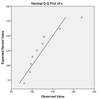
          81   95   97   101   112   125   129   167   220
3. Create the normal plot for this dataset with SPSS.
   

Random Variable Simulation

• A random variable is the process of choosing a random number.
• SPSS can generate many different types of random numbers, including from a normal distribution with a specified μ and σ.
• Example 1:   Generate 20 normal random numbers with μ = 6.7 and σ = 2.5. Here is the probability density function:
  
  
  1. Create a column with variable name i. Enter the values 1 to 20.
  2. Using SPSS, create a new variable, by selecting Transform >> Compute Variable.  Set the target variable to x and the expression to RV.NORMAL(6.7, 2.5).
• A uniform random variable with range [a,b) is a value drawn from the interval [a,b); every value in this interval is equally likely to be chosen.
• Example 2:   Generate 20 uniform random numbers from the interval [1, 3.14). Here is the probability density function:
  
  
  1. Create a column with variable name i. Enter the value 1 to 20. Here is the probability function.
  2. Using SPSS, create a new variable, by setting the target variable to y and the expression to RV.UNIFORM(1, 3.14159265). (Don't worry about why pi is used for the maximum value for the uniform random variables. It is used to show that the minimum and maximum values need not be integers.)
  3. Note: if the number of generated random numbers is large, entering the index i by hand is tedious. Here are two alternatives to Enter a Range into a Dataset. If you want to generate a column of 100 random numbers, the two alternatives are create a column of numbers from 1 to 100 are are (1) use Excel to create the column of numbers, then copy and paste it into the SPSS column, (2) run the SPSS script to generate the column of numbers.

SPSS Practice Problems

1. Create 50 values of a normal random variable x with μ = 15, σ = 3.8.
2. Create a histogram of x with superimposed normal curve.
3. Create a normal plot of x.
4. Create 50 values of a uniform random variable y in the range [10, 50].
5. Create a histogram of y with superimposed normal curve.
6. Create a normal plot of y.

Project 2

• Look at Project 2BCD.

Bivariate Datasets

Correlation

• With the Bears Roster 1985 Dataset, use SPSS to:
  
  1. Compute the height in meters and the weight in kilos of the Bears players. The conversion rates are 0.3048 meters per foot and 0.453592 kilos per pound. Use these the Compute Variable dialog to  create new variables height (Height in Meters) and weight (Weight in Kilos):
     

     Target Variable:	Label:	Numeric Expression:
     Height	Height in Meters	(HeightInFeet + HeightInInch / 12.0) * 0.3048
     Weight	Weight in Kilos	WeightInLbs * 0.453592

     
     
  2. Create the simple scatterplot of weight in kilos (y-axis) vs. height in meters (x-axis).
  3. Compute the linear correlation.

Linear Regression

• We will discuss linear regression next time on Oct 5.
• With the Bears Roster 1985 Dataset, use SPSS to:
  
  1. Compute the height in meters and the weight in kilos of the Bears players. The conversion rates are 0.3048 meters per foot and 0.453592 kilos per pound.
  2. Find the simple linear regression equation for predicting weight in kilos from height in meters.
  3. Create the residual plot, which is the residuals (y-axis) vs. the predicted values (x-axis)

Project 3

• Look at the project descriptions for Project 3AB and Project 3C.