To Notes

IT 223 -- Feb 2, 2026

Review Exercises

1. What is the total proportion (or percentage) of observations under a normal density?
   Answer: under any density including a normal one, the total area is 1, which represents the proportion 1.0 or percentage 100% of the observations.
2. Show that a normal density with a smaller spread (σ) has a taller peak so that the area under the density is always 1.  To see this, plot normal densities with center = 0 and spread equal to 1, 0.5, and 0.2. Answer:
   

   x <- seq(-4, 4, 0.005)
   y1 <- dnorm(x, mean=0, sd=1)
   plot(x, y1, type="l", ylim=c(0, 1), xlab="", ylab="", 
       main="Normal Density with Mean=0, SD=1")
   y2 <- dnorm(x, mean=0, sd=0.5)
   plot(x, y2, type="l", ylim=c(0, 1), xlab="", ylab="", 
       main="Normal Density with Mean=0, SD=0.5")
   y3 <- dnorm(x, mean=0, sd=0.2)
   plot(x, y3, type="l", ylim=c(0, 1), xlab="", ylab="", 
       main="Normal Density with Mean=0, SD=0.2")
   # Replace the previous plot with the following to view the
   # entire density:
   plot(x, y3, type="l", ylim=c(0, 2), xlab="", ylab="", 
       main="Normal Density with Mean=0, SD=0.2")
   

3. Show that a uniform density with a smaller spread (min - max) has a larger height to ensure that the total proportion (or percentage) of the observations in the interval [min, max] is always 1. Plot uniform densities with min = 0 and max = 2, 1, and 0.5. Answer:
   

   x <- seq(-1, 3, 0.005)
   y1 <- dunif(x, min=0, max=2)
   plot(x, y1, type="l", ylim=c(0, 2), xlab="", ylab="",
       main="Uniform Density with Min=0, Max=2")
   y2 <- dunif(x, min=0, max=1)
   plot(x, y2, type="l", ylim=c(0, 2), xlab="", ylab="",
       main="Uniform Density with Min=0, Max=1")
   y3 <- dunif(x, min=0, max=0.5)
   plot(x, y3, type="l", ylim=c(0, 2), xlab="", ylab="",
       main="Uniform Density with Min=0, Max=0.5")
   

4. Draw normal plots that illustrate datasets with these characteristics: (a) approximately normal, (b) skewed to the right, (c) skewed to the left, (d) thin tails, (e) fat tails.
   Answer: look at the plots in the Normal Plots document, Nonnormality Section.

Look at the Bivariate Datasets document to help you with review exercises 5, 6, and 7.

5. What is a bivariate dataset?
   Answer: a bivariate dataset is a dataset that contains two variables.
6. What is a bivariate normal dataset? Give a parsimonious description of a bivariate normal dataset.
   Answer: a bivariate normal dataset is a bivariate dataset that is normal in every direction. In particular, if x and y are the two variables in the dataset, then both x and y are normally distributed. A parsimonious description of a bivariate normal dataset requires five statistics: X, SD+_x, Y, SD+_y, and the correlation r between x and y.
7. Look at the Bears 2026 Roster: bears-2026-roster.txt. Use R to plot the weight in kilos vs. the height in meters for each player. The conversion rates are 0.3048 meters per foot and 0.4536 kilos per pound. Answer:
   

   setwd("c:/workspace")
   getwd( )
   [1] "c:/workspace"
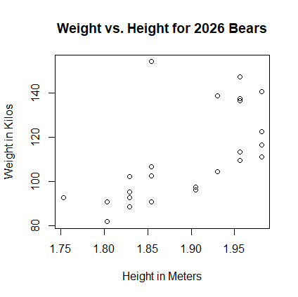
   # Create a dataframe df to hold the 2026 Bears Roster
   # First download the bears-2026-roster into 
   # the c:/workspace directory (folder).
   df <- read.csv("bears-2026-roster.txt")
   # Create data vector of players heights in meters:
   h <- (df$HtFt + df$HtIn / 12) * 0.3048
   # Create data vector of players weights in kilos:
   w <- df$Weight * 0.4536
   plot(h, w, xlab="Player Height (Meters)", 
       ylab="Player Weight (Kilos),
       main="Height and Weight of 2026 Bears Roster")
   

   
   

Correlation

• Practice Problem: With the Bears Roster 2026 Dataset, use R to compute the correlation of the height in meters vs. the weight in meters for each player. The conversion rates are 0.3048 meters per foot and 0.4536 kilos per pound.
  Answer: first execute the R statements for Problem 7 above. Then use this statement to obtain the correlation of height and weight:
  

  > cor(h, w)
  [1] 0.624795
  

Linear Regression

• Practice Problem: With the Bears Roster 2026 Dataset, use R to:
  
  1. Compute the height in meters and the weight in kilos of the Bears players. The conversion rates are 0.3048 meters per foot and 0.4536 kilos per pound.
     Answer: the R calculations to obtain the height (h) in meters and the weight (w) in kilos are shown in Problem 7 above.
  2. Find the simple linear regression equation for predicting weight in kilos from height in meters.
     Answer: Here is the R calculation:
     

     > model <- lm(w ~ h)
     
     Call:
     lm(formula = w ~ h)
     
     Coefficients:
     (Intercept)            h  
          -244.1        187.6 
     

     This means that the simple linear regression equation, sometimes known as the trend line, is
          w = 187.6 * h - 244.1

Project 3

• Look at the project descriptions for Project 3.